The spectrum of an optically thin plasma#
utu.spectrum computes the emission lines of a hot, thin plasma from
the CHIANTI atomic database, which it reads
through fiasco.
A line is worth an intensity only once the plasma emitting it is described,
so this page builds one: a column of material spread over a range of
temperatures at a fixed pressure. Out of it comes the spectrum that column
would show a spectrograph, which is how an instrument is designed around the
lines it means to observe.
The ions here are named rather than discovered.
ions() will find every ion with a line in a range of
wavelengths, but the answer depends on which ions the database at hand
describes, and the one these pages are built against describes only a few.
Naming them keeps this page saying the same thing wherever it is run.
import astropy.units as u
import fiasco
import matplotlib.pyplot as plt
import named_arrays as na
import numpy as np

import utu

# fiasco says which approximations it has fallen back on for each ion,
# which is worth reading once and not seven times
fiasco.log.setLevel("ERROR")
Naming ions#
CHIANTI names an ion by its element and its charge state, counting from one,
so that the neutral atom is 1. Spectroscopists write the same thing with
a Roman numeral, and spectroscopic() translates between
the two. It takes a name or an array of them.
ion = ["He 1", "O 3", "O 4", "O 5", "Ne 7", "Mg 10", "Si 11"]

[utu.spectrum.spectroscopic(i) for i in ion]
['He I', 'O III', 'O IV', 'O V', 'Ne VII', 'Mg X', 'Si XI']
The plasma#
The plasma is described by three arrays which share an axis of temperature.
The density follows from the temperature and a pressure, since the corona is
near enough to hydrostatic that the two are not independent. Giving the
density the axis name of the temperature is what says so:
utu.spectrum reads a density on the axis of the temperature as one
density per temperature, and a density on an axis of its own as every density
at every temperature.
The emission measure is how much material there is at each temperature, \(\int n_e^2 \, dh\) through the column. A real one is measured; this one is a Gaussian in \(\log T\) centred where the transition region emits, holding \(10^{27}\,\mathrm{cm}^{-5}\) of material in all.
axis = "temperature"

temperature = na.geomspace(1e4, 1e7, axis=axis, num=61) * u.K

pressure = 1e15 * u.K / u.cm ** 3
density = pressure / temperature

weight = np.exp(-np.square((np.log10(temperature / u.K) - 5.8) / 0.3) / 2)
emission_measure = 1e27 / u.cm ** 5 * weight / weight.sum(axis)

emission_measure.sum(axis)
ScalarArray(
    ndarray=1.e+27 1 / cm5,
    axes=(),
)
Contribution functions#
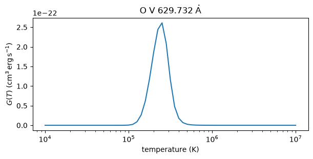
The contribution function \(G(T)\) of a line is the power it radiates per unit emission measure, and it is sharply peaked: a line is emitted only by plasma near the temperature at which its ion exists at all. This is what makes a line a thermometer, and what makes the choice of a passband a choice about which part of the atmosphere to look at.
contribution_function() returns every line of one ion at
once, as a function of wavelength, so that a line and its strength cannot
come apart.
result = utu.spectrum.contribution_function(
    ion=fiasco.Ion("O 5", temperature.ndarray),
    density=density,
    axis_temperature=axis,
)

result.outputs.shape
{'temperature': 61, 'line': 2995}
The strongest of them is the line at 629.7 Å, the line ESIS was built to observe, and it is emitted at a quarter of a million kelvin.
index = np.argmax(result.outputs.max(axis), axis="line")

fig, ax = plt.subplots(figsize=(6, 3), constrained_layout=True)
na.plt.plot(temperature, result.outputs[index], ax=ax, axis=axis)
ax.set_xscale("log")
ax.set_xlabel(f"temperature ({temperature.unit:latex_inline})")
ax.set_ylabel(f"$G(T)$ ({result.outputs.unit:latex_inline})")
ax.set_title(
    f"{utu.spectrum.spectroscopic('O 5')} "
    f"{result.inputs[index].ndarray:latex_inline}"
);
The lines#
lines() does this for every ion given to it, weights each
contribution function by the emission measure, sums over temperature, and
returns what is left brightest first. The wavelength and the ion of a line
are components of the inputs, and its intensity is the output, so that
sorting or selecting lines carries all three together.
result = utu.spectrum.lines(
    temperature=temperature,
    density=density,
    emission_measure=emission_measure,
    wavelength_min=550 * u.AA,
    wavelength_max=680 * u.AA,
    ions=ion,
)

result.shape
{'line': 1136}
The emission is isotropic, so the radiance of a line is its intensity spread over the whole sphere.
num = 8
brightest = result[{"line": slice(num)}]

radiance = brightest.outputs / (4 * np.pi * u.sr)
radiance = radiance.to(u.erg / u.s / u.cm ** 2 / u.sr)

name = utu.spectrum.spectroscopic(brightest.inputs.ion)
wavelength = brightest.inputs.wavelength

print(f"{'ion':>6s}{'wavelength':>14s}{'radiance':>14s}")
for i in range(num):
    j = {"line": i}
    print(f"{name[j].ndarray:>6s}"
          f"{wavelength[j].ndarray.to_value(u.AA):>14.2f}"
          f"{radiance[j].ndarray.value:>14.1f}")
   ion    wavelength      radiance
   O V        629.73        2652.8
  O IV        554.51         387.0
  O IV        554.08         150.4
  O IV        609.83         117.3
  Mg X        609.79         109.7
  O IV        555.26          77.9
  O IV        553.33          77.4
  O IV        608.40          63.3
The spectrum#
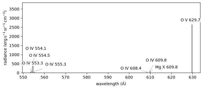
Drawn as a stem from zero for each line, this is the picture an instrument is
designed against: where the light is, and how much of it there is beside
everything else the passband will admit.
stem() draws it and names the brightest lines, moving the
labels apart so that none covers another or crosses a line it does not belong
to.
It takes a spectrum in the shape lines() returns, so the
radiance computed above has to be put back into one before it can be drawn.
fig, ax = plt.subplots(figsize=(7, 3), constrained_layout=True)
utu.spectrum.stem(
    na.FunctionArray(inputs=brightest.inputs, outputs=radiance),
    ax=ax,
)
ax.set_xlabel(f"wavelength ({u.AA:latex_inline})")
ax.set_ylabel(f"radiance ({radiance.unit:latex_inline})");